Applications IV // Neato Soccer
Today
- Application III Discussion: Human-Robot Collaboration: Search and Rescue
- Neato Soccer + Project Proposal Check-Ins + Studio
For Next Time
- Read over the Broader Impacts assignment Part 2, due on November 4th at 7PM
- In class discussions on Monday November 3rd
- Read over the Machine Vision Project Document.
- Project Proposal is due on Wednesday October 22nd at 9PM
- Project Shareouts will be Monday November 10th in class
- Project Materials are due on Tuesday November 11th at 7PM
- Consider whether there is feedback you’d like to share about the class
Applications III: Human-Robot Collaboration: Search and Rescue
We’re going to be discussing a new topic related to the broader applications of robotics: human-robot collaboration. This is a vast space, which covers anything from humans using robots as extensions of themselves (as tools), to humans and robots interacting as equals on collaborative or cooperative teams.
Today, we’re going to start thinking about human-robot collaboration in the context of one of the most cited “uses” of semi-intelligent robotics in modern academic literature: search and rescue. As your discussion unfolds, please fill in this survey.
A Scan of the Literature
In your table groups, open the following link to some open-source “Search and Rescue” academic literature. Each person should choose a different paper to skim (please don’t read the papers in complete detail!).
As each person skims, take note of the following:
- Is what is being sought named in the paper?
- Is the robot discussed “real” (as in, exists in the world)?
- Is the robot deployed in a “real” environment (as in, is it fully simulated, in a laboratory, or field tested)?
- When referring to “search and rescue” what other applications may be listed? Or what specific organizations or scenarios are mentioned, if any?
- Who funded the work?
- Is the robot or robot system mostly a “searcher” or a “rescuer”?
- Do the papers make mention of how human operations specialists will interact with the robot?
After you’ve each had an opportunity to skim, share out your results. Pay special attention to where there are similarities or differences between your robots. You might want to identify a few axes and map your different robots to these axes (please use the board for this!).
Intended Use
As you might notice in the first activity, the landscape of Search and Rescue robots can be quite broad – from clearly bespoke solutions to specific scenarios/teams, to general purpose robots. The latter cases are particularly interesting – what makes a search and rescue robot…a search and rescue robot, if not its form/functionality?
There are multiple ways in which a technology is operationalized for a particular use case:
- By fundamental design (e.g., the form or functionality is entirely niche)
- By licensing or IP controls (e.g., commercial, non-commercial, open-source, closed-source)
- By market controls (e.g., only selling to certain buyers, lease/renting/buying models)
- By partnership (e.g., robots are provided only to trusted partners, potentially with a point-of-contact or dedicated engineer to monitor use)
- Maybe others! (if you can think of some, let us know and we can add them here)
For these search and rescue robots you just discussed, consider the following in your groups:
- Can algorithms be designed to restrict their utility to these search and rescue applications; why or why not?
- In what way is an engineer responsible for considering unintended use of their system? What actions should they take (or not)?
- Assuming that an algorithm is free to use, what evidence should be provided that it works as expected? How should limitations of the algorithm be communicated?
Setting Standards for SAR
In the US, the Federal Emergency Management Agency (FEMA), Homeland Security, and the Department of Defense are among the largest customers of SAR robots. In partnership with NIST (the National Institute of Standards and Technology), the guidelines for an effective/useable SAR system for urban environments has been defined (you can read more here) and covers the following:
- Human-System Interaction (23 requirements)
- Logistics (10 requirements)
- Operating Environment (5 requirements)
- System (physical robot) (65 requirements; 32 of which are for sensing)
One of the fascinating things about these requirements is that “Human-System Interaction” primarily covers the robot operator but not the interaction with a possible human rescuee. In your small groups, consider the following questions from the perspective of a NIST engineer tasked with setting requirements for a SAR robot (I recommend picking one or two to focus on):
- What would/should official standards for Human-System Interaction cover for the rescuee of a SAR robot?
- You may want to consider: interfaces (virtual, sensory, or physical); accessibility; meta-safety; inclusivity…
- How would these standards interact with your robot’s sensors? Algorithms?
- You may want to consider: role of automation/autonomy; consequences of perceptual limitations; edge-cases for perception choices; introduction of bias (implicit or explicit); verifiability; explainability…
- Who should be involved in co-designing this set of standards for this group of stakeholders?
- The current standards were set based on several workshops with experts in the field (peep the list in the linked report above…notice anything interesting about this group?)
- What tests would need to be designed to assess whether a robot met these standards?
Neato Soccer
This activity is designed to get you up-and-running with OpenCV and ROS with our Neatos to implement a simple sensory-motor loop using image inputs. Let’s play some soccer!
Connect to a Neato
Grab a Neato with your table group – make sure you pick one of the Neatos with a camera attachment on it.
$ ros2 launch neato_node2 bringup.py host:=ip-of-your-neato
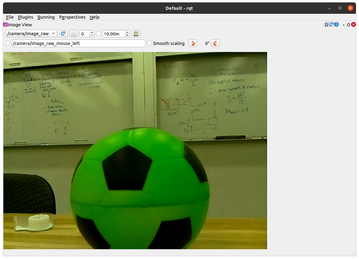
You can visualize the images coming from the camera using rqt. First launch rqt.
$ rqt
Next, go to Plugins, then Visualization, and then select Image View. Select /camera/image_raw from the drop down menu. If you did this properly you should see something like the following on your screen:
OpenCV and Images as Arrays
We’re created from starter code in the class_activities_and_resources repository. (Be sure to pull from upstream to get the latest!) which you may want to use for this activity. Specifically, you want to look in the neato_soccer package and modify the node called ball_tracker.py.
Activity: Have a look at
ball_tracker.py– what is being subscribed to? What libraries are being used? What is the architecture of the node?
The starter code leverages the OpenCV library to handle images; currently the node subscribes to an image topic, and then uses the cv_bridge package to convert from a ROS image message to an OpenCV image.
An OpenCV image is just a numpy array. If you are not familiar with numpy, you may want to check out these tutorials: numpy quickstart, numpy for matlab users. Since an image is just an array, you can perform all sorts of standard transformations on your image (rotation, translation, kernel convolutions) just like you would any other matrix!
Run the starter code and you’ll see the dimensionality of the numpy array of your image printed out from process_image. You’ll notice that the encoding of the image is bgr8 which means that the color channels of the 1024x768 image are stored in the order blue first, then green, then red. Each color intensity is an 8-bit value ranging from 0-255.
If all went well, you should see an image pop up on the screen that shows both the raw camera feed as well as a color filtered version of the image.
Note: do pay attention to how OpenCV is being used in your node to generate visualizations. A very easy bug to introduce into your Opencv code is to omit the call to the function
cv2.waitKey(5). This function gives the OpenCV GUI time to process some basic events (such as handling mouse clicks and showing windows). If you remove this function from the code above, check out what happens.
Filtering Based on Color
We want to identify our soccer balls in our streaming images from the Neato. There are many, many, many ways this could be done, but for the purposes of this activity, we’ll be performing color-based filtering.
In the starter code, the color filtering image is produced using the cv2.inRange function to create a binarized version of the image (meaning all pixels in the binary image are either black or white) depending on whether they fall into the specified range. As an example, here is the code that creates a binary image where white pixels would correspond to brighter pixels in the original image, and black pixels would correspond to darker ones
self.binary_image = cv2.inRange(self.cv_image, (128,128,128), (255,255,255))
This code could be placed inside of the process_image function at any point after the creation of self.cv_image. Notice that there are three pairs lower and upper bounds. Each pair specifies the desired range for one of the color channels (remember, the order is blue, green, red). If you are unfamiliar with the concept of a colorspaces, you might want to do some reading about them on Wikipedia!
Activity: Your next goal is to choose a range of values that can successfully locate the ball. In order to see if your
binary_imagesuccessfully segments the ball from other pixels, you should visualize the resultant image using thecv2.namedWindow(for compatibility with later sample code you should name your windowbinary_image) andcv2.imshowcommands (these are already in the file, but you should use them to show your binarized image as well).
Debugging Tips
Any interaction with Opencv’s GUI functios (e.g., cv2.namedWindow or cv2.imshow) should only be done inside of loop_wrapper or run_loop functions (this is because you want to interact with the UI of OpenCV from the same thread).
White pixels will correspond to pixels that are in the specified range and black pixels will correspond to pixels that are not in the range (it’s easy to convince yourself that it is the other way around, so be careful).
We have added some code so that when you hover over a particular pixel in the image we display the r, g, b values. If you are curious, we do that using the following line of code.
cv2.setMouseCallback('video_window', self.process_mouse_event)
We then added the following mouse callback function.
    def process_mouse_event(self, event, x,y,flags,param):
        """ Process mouse events so that you can see the color values
            associated with a particular pixel in the camera images """
        image_info_window = 255*np.ones((500,500,3))
        cv2.putText(image_info_window,
                    'Color (b=%d,g=%d,r=%d)' % (self.cv_image[y,x,0], self.cv_image[y,x,1], self.cv_image[y,x,2]),
                    (5,50),
                    cv2.FONT_HERSHEY_SIMPLEX,
                    1,
                    (0,0,0))
One piece of good practice when using OpenCV – especially as you are learning! – is to use interactive GUI elements to set your function values. Here, you may want to add sliders to set your lower and upper bounds for each color channel interactively.
If you’re using ROS, you could alternatively use ROS parameters and
dynamic_reconfigure(e.g., see this example).
To create an interactive GUI in OpenCV in ROS, you’ll want to make some new functions and “callbacks” in your Node. First, add the following lines of code to your loop_wrapper function:
        cv2.namedWindow('binary_image')
        self.red_lower_bound = 0
        cv2.createTrackbar('red lower bound', 'binary_window', self.red_lower_bound, 255, self.set_red_lower_bound)
This code will create a class attribute to hold the lower bound for the red channel, create the thresholded window, and add a slider bar that can be used to adjust the value for the lower bound of the red channel. The last line of code registers a callback function to handle changes in the value of the slider (this is very similar to handling new messages from a ROS topic). To create the call back, use the following code:
    def set_red_lower_bound(self, val):
        """ A callback function to handle the OpenCV slider to select the red lower bound """

        self.red_lower_bound = val
All that remains is to modify your call to the inRange function to use the attribute you have created to track the lower bound for the red channel.
Remember the channel ordering! In order to fully take advantage of this debugging approach you will want to create sliders for the upper and lower bounds of all three color channels.
Here is what the UI will look like if you add support for these sliders.
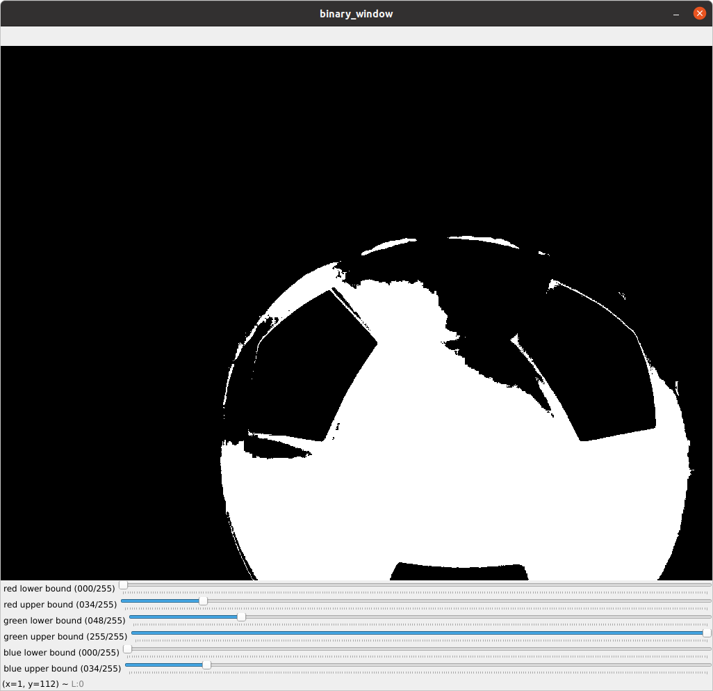
The code that generated this visual is included in the neato_soccer package as ball_tracker_solution.py. You can run it through the following command.
$ ros2 run neato_soccer ball_tracker_solution
If you find the video feed lagging on your robot, it may be because your code is not processing frames quickly enough. Try only processing every fifth frame to make sure your computer is able to keep up with the flow of data.
An Alternate Colorspace
Separating colors in the BGR space can be difficult. To best track the ball, you could consider using the hue, saturation, value (or HSV) color space. See the Wikipedia page for more information. One of the nice features of this color space is that hue roughly corresponds to what we might color while the S and the V are aspects of that color. You can make a pretty good color tracker by narrowing down over a range of hues while allowing most values of S and V through (at least this worked well for me with the red ball).
To convert your RGB image to HSV, all you need to do is add this line of code to your process_image function.
self.hsv_image = cv2.cvtColor(self.cv_image, cv2.COLOR_BGR2HSV)
Once you make this conversion, you can use the inRange function the same way you did with the BGR colorspace. You may want to create two binarized images that are displayed in two different windows (each with accompanying sliders bars) so that you can see which works better.
Dribbling the Ball
There are probably lots of good methods for controlling your Neato to interact with the ball, but we suggest using a simple proportional controller that considers the “center of mass” of your filtered image to set the angle that the Neato should turn to move towards the ball as a good first step…
Tips for Playing Ball
To compute the center of mass in your binarized image, use the cv2.moments function. Take a second to pull up the documentation for this function and see if you can understand what the code below is doing. You can easily code this in pure Python, but it will be pretty slow. For example, you could add the following code to your process_image or run functions.
        moments = cv2.moments(self.binary_image)
        if moments['m00'] != 0:
            self.center_x, self.center_y = moments['m10']/moments['m00'], moments['m01']/moments['m00']
When doing your proportional control, make sure to normalize self.center_x based on how wide the image is. Specifically, you’ll find it easier to write your proportional control if you rescale self.center_x to range from -0.5 to 0.5. We recommend sending the motor commands in the self.run function.
If you want to use the sliders to choose the right upper and lower bounds before you start moving, you can set a flag in your __init__ function that will control whether the robot should move or remain stationary. You can toggle the flag in your process_mouse_event function whenever the event is a left mouse click. For instance if your flag controlling movement is should_move you can add this to your process_mouse_event function:
        if event == cv2.EVENT_LBUTTONDOWN:
            self.should_move = not(self.should_move)